Uncategorized
Diesel Fuel Details
The big story during August and September was Hurricane Harvey. At its worst, Harvey knocked about 20% of U.S. refining capacity knocked offline. As a result the average price of regular gasoline jumped by 34-cents per gallon (15%) between the end of July to the week of September 11th, when it peaked at $2.61 per gallon. The price of diesel increased also rose by 27-cents per gallon (10.7%).
Crude oil prices actually fell as the storm hit Houston. During August the WTI price dropped from $50.21 per bbl to $45.96 per bbl. But since the beginning of September the WTI price has recovered, hitting $49.88 on the 18th. Going along with the crude oil price fluctuations, the U.S. crude oil inventory dropped by 19.8 million barrels (1.7%) during August, but risen since the beginning of September by 11.6 million barrels.
During August the price of Brent crude rose slightly from $51.99 to $52.69 per bbl. Data on domestic oil production and imports are only available through June. That month domestic producers accounted for 53.2% of the U.S. oil supply, and domestic production averaged 9.1 bbl per day. Shale oil accounted for 52.5% of domestic production.
Turning to domestic motor fuel consumption, for which the most current data is from last April, gasoline consumption totaled 12.0 billion gallons, up 206.5 million gallons (1.7%) from the prior April. This is a notable increase&mdashover the most recent three months gasoline consumption had declined by 0.2%.
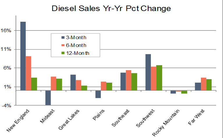
Diesel fuel consumption in April totaled 3.4 billion gallons, up 153.2 million gallons (4.7%) from April 2016. During the prior 3-, 6- and 12-month diesel fuel consumption grew by 3.7%, 4.3% and 3.6%, compared to the same periods in the prior year.
Regionally, over the three months from February&mdashApril the strongest growth occurred in New England states (18.3%) followed by the Southwest states (9.7%). States in the Southeast, Great Lakes and Far West regions also experienced some growth, but below 5.0% in all cases. The greatest decline occurred in the Mideast states (-3.9%). Other regions where diesel fuel consumption decreased included the Plains (-2.0%) and the Rocky Mountains (-0.8%). The states of the Rocky Mountain region have experienced year-over-year declines during the most recent 3-, 6- and 12-month periods.
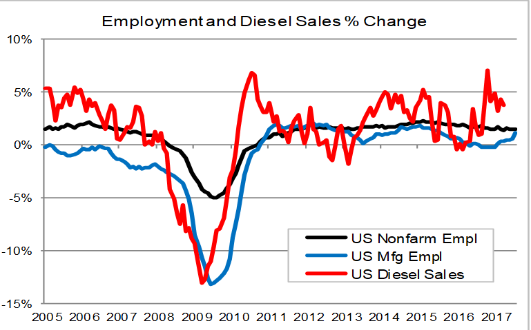
As shown on the above graph, the relationship between the 3-month moving average of diesel fuel sales and manufacturing employment continues to hold. However, the number of months by which changes in the diesel series leads the manufacturing employment series does fluctuate. The diesel series started becoming increasingly positive in March 2016, while the growth rate for manufacturing employment stayed negative until February 2017. Manufacturing employment growth has stayed positive and has continued to increase over the past seven months with a large jump from July (0.6%) to August (1.1%). If the relationship continues to hold, the year-over-year manufacturing employment growth rate will likely level off at about 1.3% for the remainder of 2017.
Just around the Corner? Maybe Not.
A very smart analyst joked yesterday that the Consumer Price Index is the new Nonfarm Payroll. Since the FOMC has made it clear that they are waiting for 2% inflation—or perhaps Godot—all eyes are searching for signs we might be getting there, so all price indexes are good fodder, especially the PCE, the Fed’s favored index.
The FOMC’s models have continually demonstrated a “just around the corner,” feature where, despite currently weak PCE measures, the expectation is that higher inflation would occur in the near future.
Unfortunately, a historical look at the broad components of this inflation measure belies their optimistic projections:
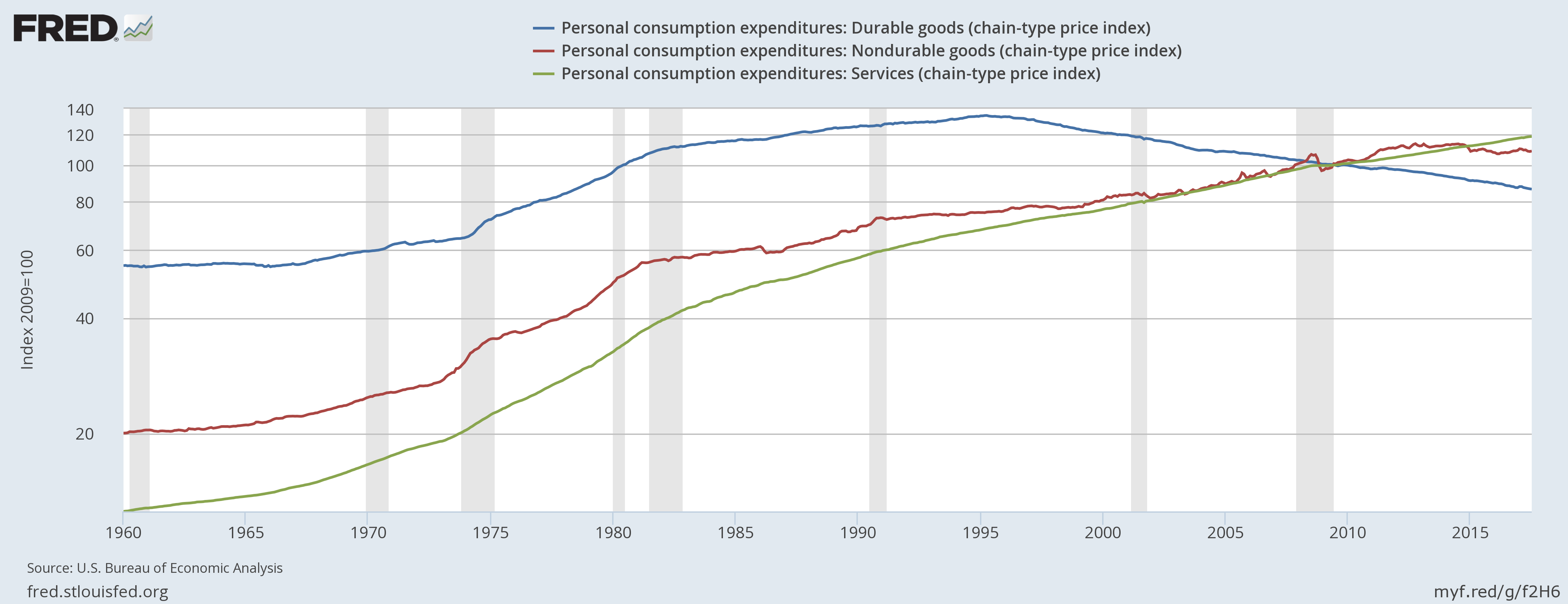
Above is a logarithmic graph of the three components of the PCE price index: durable goods prices (in blue), non-durable goods prices (in red) and service prices (in green). Two key visual elements are apparent: durable goods prices have been consistently declining since the mid-1990s. Non-durable goods prices have been stagnant to slightly lower for the last 5 years. That leaves services as the only PCE price index component that can exert upward pressure.
Let’s look at the same data from a Y/Y percentage change perspective:
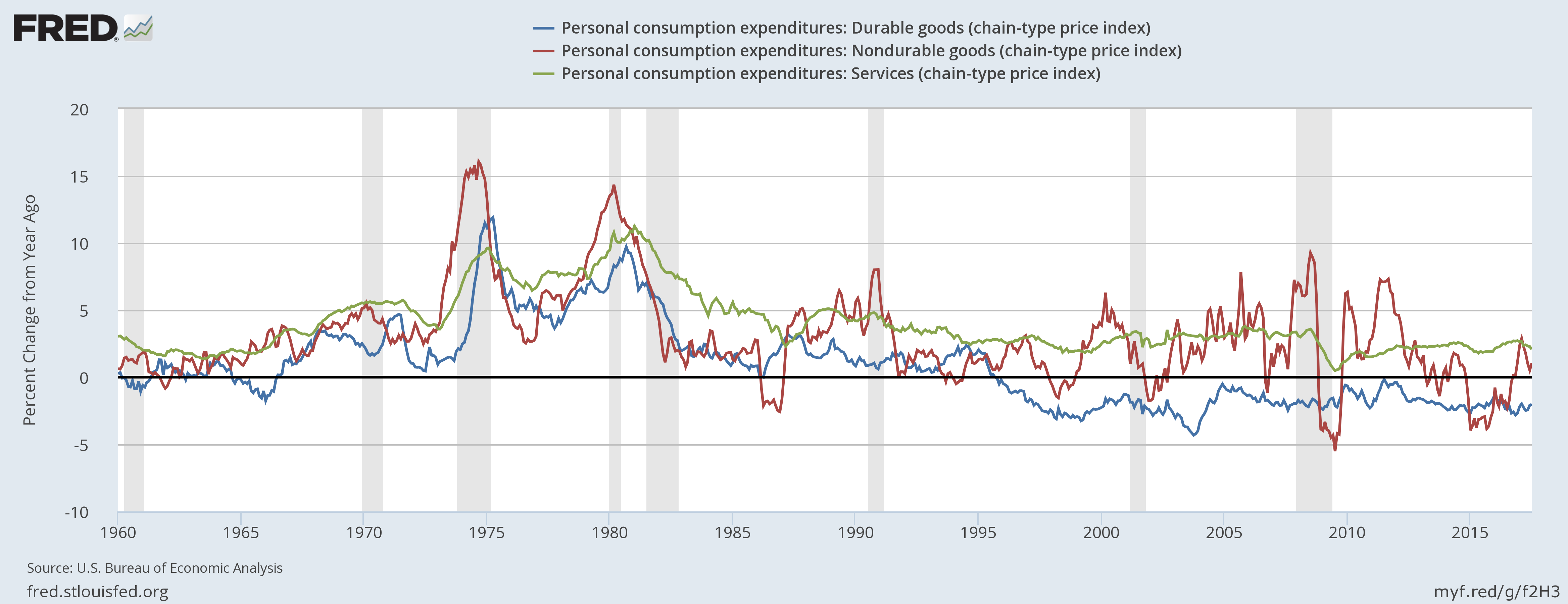
Durable goods prices (in blue) have been subtracting from price growth for the last 20 years. Non-durable goods prices (in read) have been declining since 2011-2012; they subtracted from PCE price growth for most of 2015 and only recently turned positive. Only service prices (in green) have increased PCE price pressures on a consistent basis.
There are several important lessons to draw from this data. First, the PCE price index looks at prices from a business perspective. According to the Cleveland Fed, “the PCE is based on surveys of what businesses are selling.” The above charts indicate that neither durable goods nor non-durable goods companies have any pricing power. Second, the Y/Y percentage change in service prices has been declining. Third, price growth for 31% of PCEs are either negative or very weak. That means the remaining 70% of prices would have to increase at a faster Y/Y rate to hit the Fed’s 2% PCE Y/Y inflation target. This runs counter to the second conclusion regarding service prices, that the y/y rate of change is narrowing.
Those trends mean the Fed cannot hit its 2% y/y target under the current circumstances.
State-level GDP: Down on the Farm with Energy Rising
During first quarter of 2017, economic growth declined in five of the seven Plains states. Within this region, only Missouri and North Dakota saw their economies grow during the quarter. North Dakota’s growth came from a reviving energy sector that contributed 1.7pp and offset almost the entire 1.9pp drop in its agriculture sector. Missouri’s agriculture sector declined by 0.8pp, but this was offset by relatively strong growth in durable goods manufacturing and wholesale trade.
The states that experienced the greatest declines in output were Nebraska (-4.0%), South Dakota (-3.8%), and Iowa (-3.2%). Lower prices for row crops likely explain the decline. During the first quarter of 2017 corn prices averaged 4.4% below the prior year and wheat prices were down 11.7%. Soybean prices were up somewhat compared to 2016 but were trending lower.
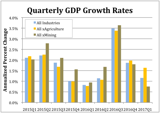
Nationwide the agriculture, forestry, fishing and hunting sector subtracted 0.41pp from the overall annualized growth, which totaled 1.1%. As the accompanying chart shows, absent the agriculture sector national GDP grew by 1.6% during the first quarter.
The fasted growing sector in Q1 was mining, which includes oil extraction. It was up 0.3%. As shown in the accompanying chart, excluding the mining sector national GDP would have only increased by 0.8%.
Texas 3.9% gain was the strongest. Its mining sector increased by 2.1pp. West Virginia experienced the second highest rate of overall growth at 3.0% and its mining sector contributed 3.2pp. New Mexico had the third highest growth rate at 2.8% with its mining sector contributing 1.8pp. Other energy states also experienced increased growth. Oklahoma’s 1.9% growth in output ranked 11th and noisy Alaska’s 1.8% growth ranked 14th. (A revenue estimator from the state told us they basically don’t even try to forecast revenue growth in the state because the economy is so volatile.)
But other energy states did not fare as well. Lousiana’s economy grew by only 1.0% (ranked 28th). Growth in Wyoming clocked at just 0.9% (32nd), and Montana saw a 0.5% decline (45th)
Finally, a couple of standout states for the quarter were Washington and Wisconsin. Washington continued a pattern of strong performance from 2016 when it took the blue ribbon. Its economy grew at an annualized rate of 2.7% during the first quarter and by 3.8% for all of 2016. This growth was driven by its information sector, which accounted for 1.7pp, and durable goods manufacturing, which accounted for 0.7pp, of the overall growth. Wisconsin’s 2.1% annualized growth for the first quarter represents a reversal of fortune from 2016 during, when its economy grew by only 0.9%. The sectors that contributed the most to its first quarter 2017 growth were real estate (0.6pp), durable goods manufacturing (0.4pp) and nondurable goods manufacturing (0.4pp).
Subscriptions
No ideology, no agenda, just a straight take on breaking economic data.
Each week as we scrutinize incoming data, we will send you a graph and a concise note on anything new that’s worth your time, 4 – 5 times a week. Our perspective allows you to make intelligent decisions no matter what political or economic outlook you embrace.
Subscribe for $27 a month > More Info...
Subscribe >
More Info...
Subscribe >
 More Info...
Subscribe >
More Info...
Subscribe >